Multi-Resolution Shared Representative Filtering for
Real-Time Depth Completion
Yu-Ting Wu1
Tzu-Mao Li2
I-Chao Shen3
Hong-Shiang Lin4
Yung-Yu Chuang1
National Taiwan University1 MIT CSAIL2 The University of Tokyo3 FIH Mobile Limited4
Interactive Comparison on Synthetic and Real-World Data
Image viewer is borrowed from this page.
All results are generated on a machine with Intel Core i5-7400K at 3.0 GHz, 16-GB of RAM, and an NVIDIA GeForce GTX 2080 Ti graphics card.
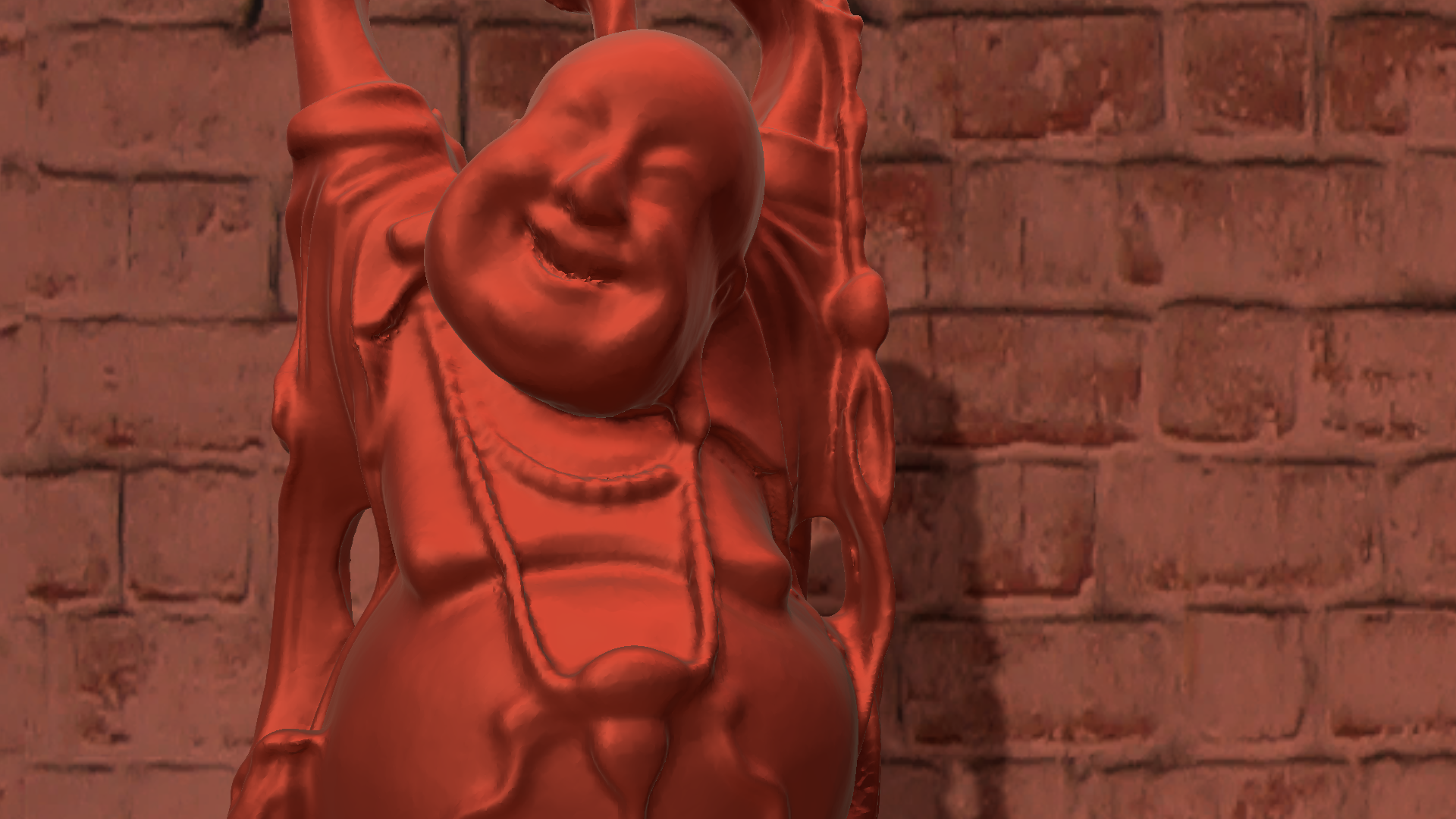
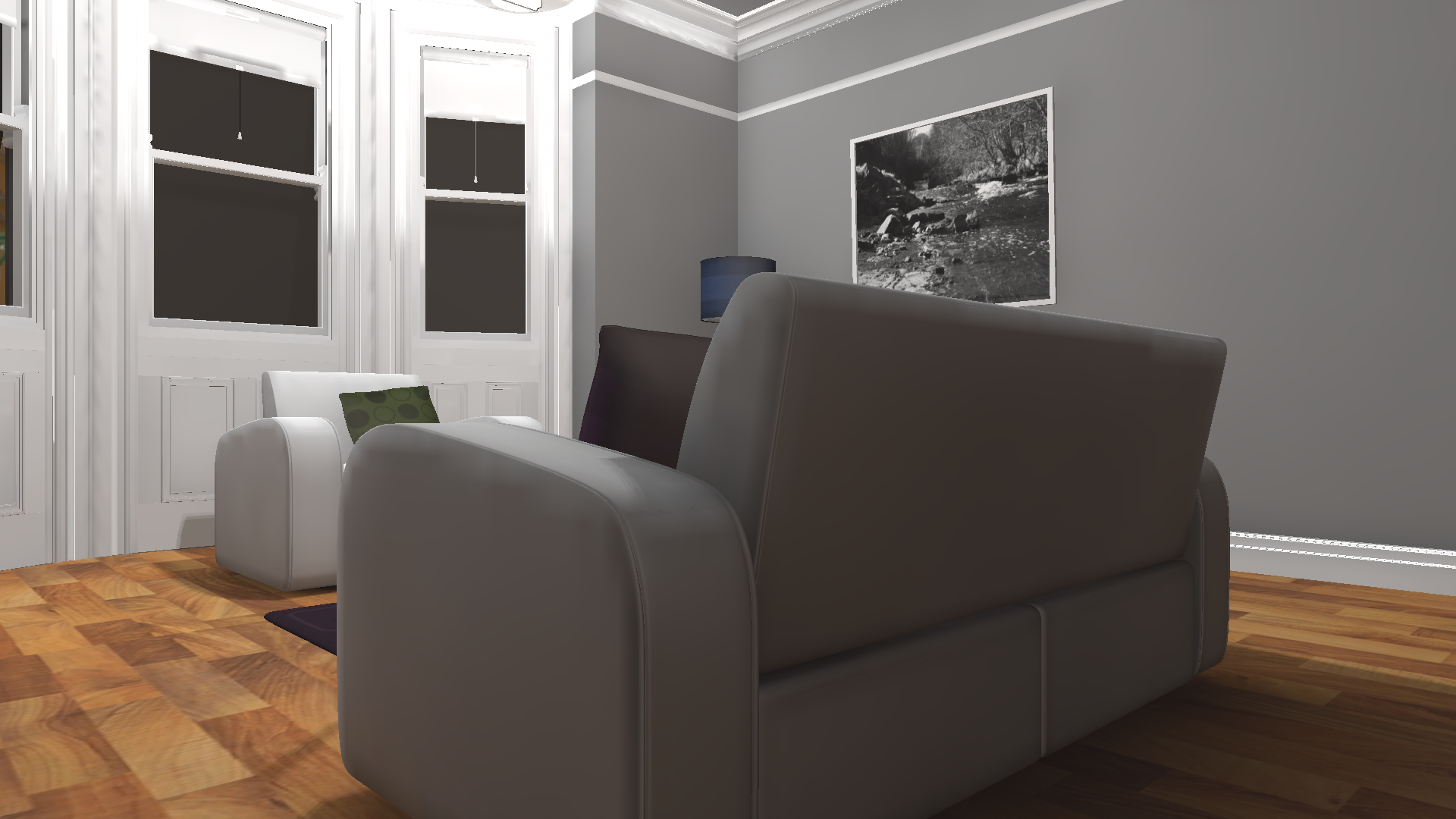
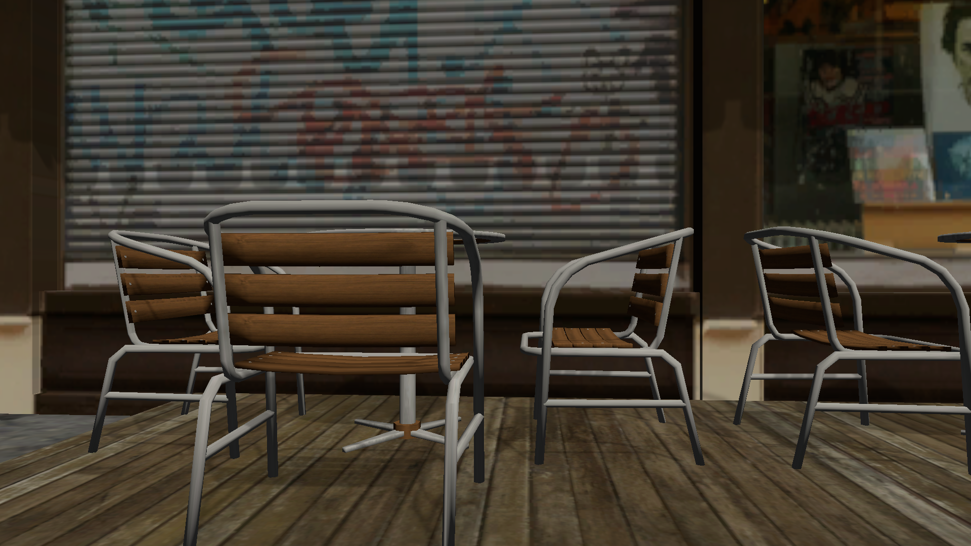
Synthetic Scenes (click on the thumbnail to select the scene comparison shown at the bottom of the page)
 |
 |
 |
 |
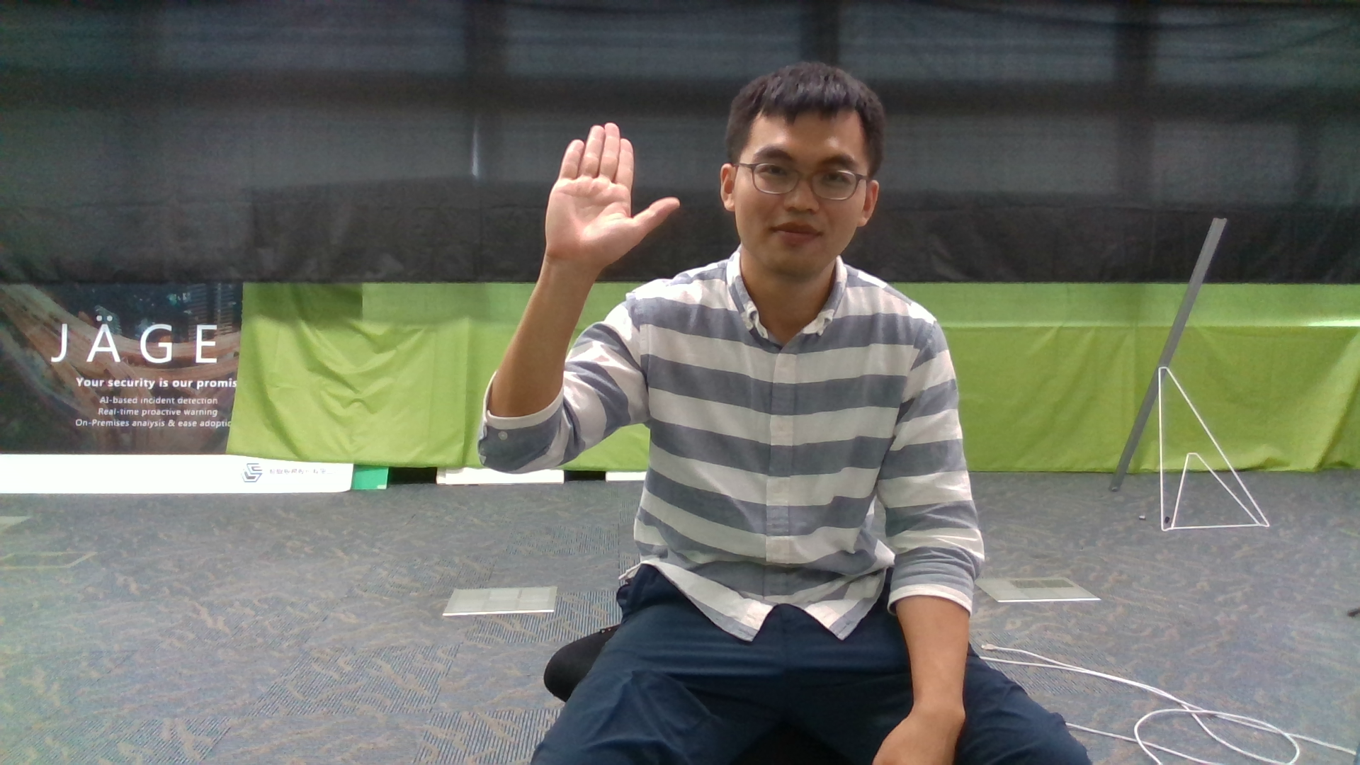
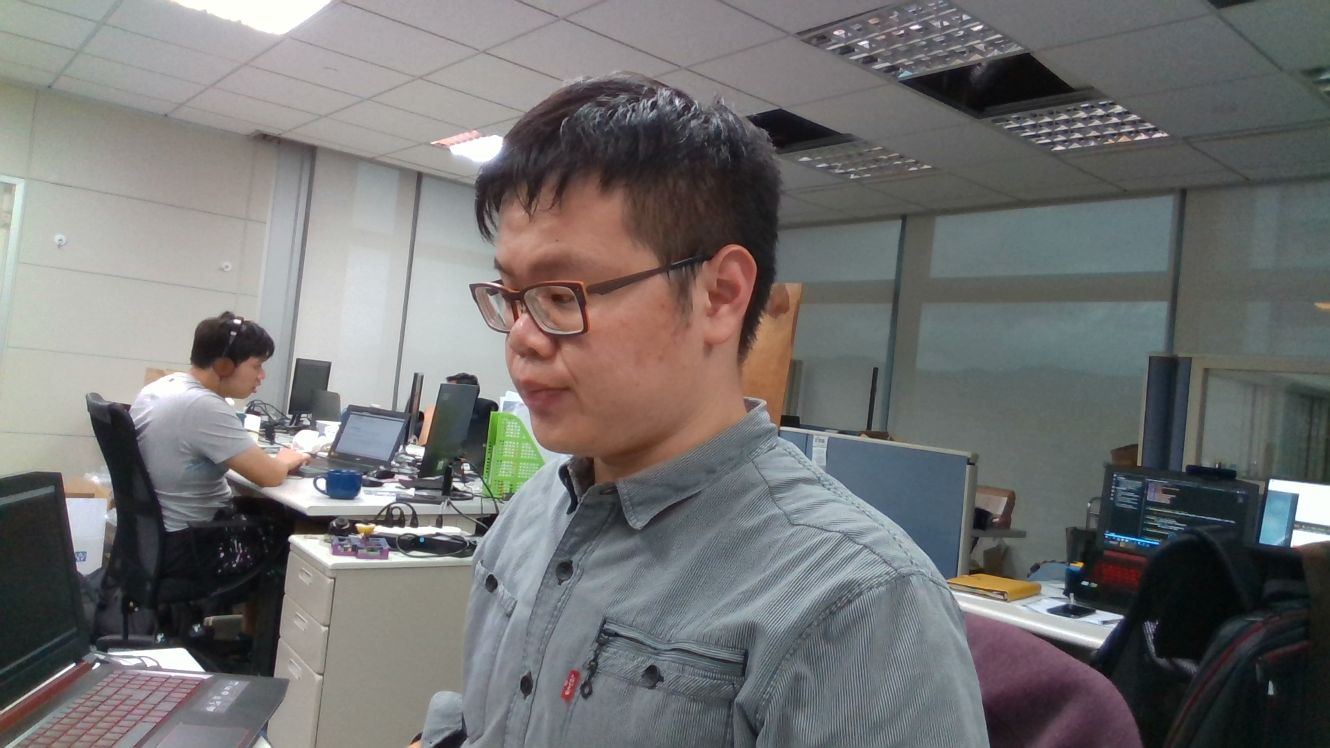
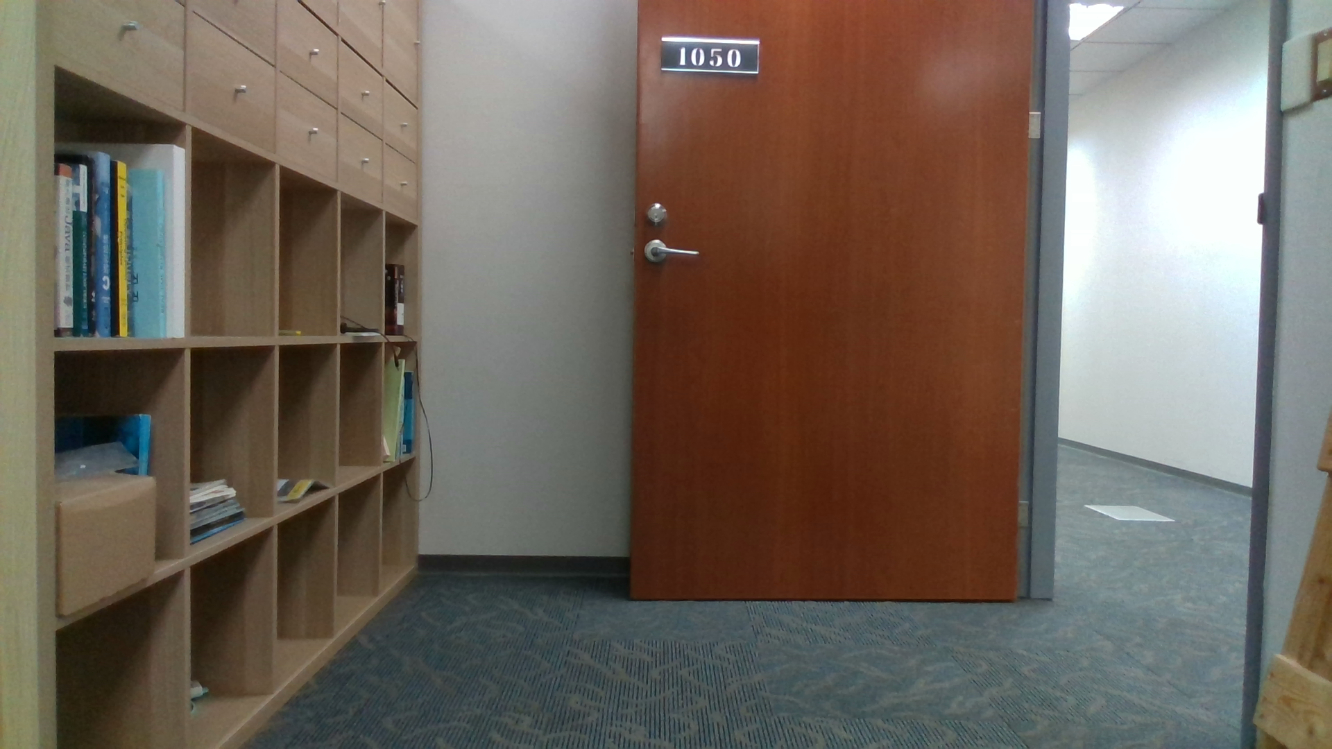
Real-World Scenes (click on the thumbnail to select the scene comparison shown at the bottom of the page)
Captured by Intel RealSense D-435
 |
 |
 |
 |
Compared Methods
Joint Bilateral Filtering (JBF) [Kopf et al. 2007]
Shared Representative Filtering (SRF) [Our method]
Multi-Res. Joint Bilateral Upsampling (M-JBU) [Richardt et al. 2012]
Fast Bilateral Solver (FBS) [Barron and Poole 2016]
Multi-Res. Shared Representative Filtering (M-SRF) [Our method]
Implementation and Time Budgets
Joint Bilateral Filtering [Kopf et al. 20007], Multi-Res. Joint Bilateral Upsampling [Richardt et al. 2012] and our methods (SRF and M-SRF) are implemented with Unity shaders, running on GPU.
We allocated 15.0 ms. for single-resolution methods (JBF and SRF) and 7.5 ms. for multi-resolution methods (M-JBU and M-SRF) as time budget to complete the depth map.
For Fast Bilateral Solver [Barron and Poole 2016], we use the authors' CPU python implementation. It takes about 300 ~ 500 ms.
Mean Absolute Error (MAE) and Peak Signal-to-Noise Ratio (PSNR)
| Method | JBF | SRF | M-JBU | FBS | M-SRF |
| MAE | N/A | 0.0399 | 0.0654 | 0.0511 | 0.0308 |
| PSNR | N/A | 29.19 | 26.02 | 29.77 | 31.71 |